
Derivative-Informed Neural Operators
Check out a short GitHub tutorial here!
Derivative-informed operator learning enriches operator approximation with derivative information, improving accuracy and sample efficiency for maps between function spaces. This idea applies broadly to scientific maps whose derivatives are informative or efficiently available, including maps defined by simulators, optimization problems, inverse problems, and dynamical or PDE models. Derivative-informed neural operators (DINOs) instantiate this principle with neural operators.
Conventional neural operator training
Neural operators are neural network surrogates for maps on function spaces, where the neural network parametrization is independent of a specific numerical discretization of the target map. They are useful whenever the object being learned is an operator rather than a finite-dimensional vector-to-vector map; parametric PDE solution maps are a central example. Neural operators are typically trained in the \(L^2_\mu\) parametric Bochner space.
\[\min_w \mathbb{E}_{m \sim \mu}\left[\|u(m) - u_w(m)\|^2_{\mathcal{U}} \right]\]DINO training
Derivative-informed neural operators (DINOs) are neural operators that are trained to learn both an operator and its (Fréchet) derivatives, that is the training is formulated in the \(H^1_\mu\) Bochner space (or \(H^k_\mu\) with \(k\in \mathbb{N}\)).
\[\min_w \mathbb{E}_{m \sim \mu}\left[\|u(m) - u_w(m)\|^2_{\mathcal{U}} + \|\mathcal{D}u(m) - \mathcal{D}u_w(m)\|^2_{HS(\mathcal{M},\mathcal{U})} \right]\]The key issue for DINO is to devise representations of the neural operator and the training problem that lead to efficient representations of the derivative \(\mathcal{D}u\), which leads to efficient offline computation of training data and efficient DINO training.
Advantages of DINO
Improved generalization per unit compute
Derivatives (e.g., Jacobians) of operator maps can often be computed, approximated, or compressed at a significantly lower cost when compared to the function output itself. This happens in many settings, including implicit models, adjoint-enabled simulators, and time-stepping methods. As a concrete example, consider an implicitly defined parametric PDE map in a strong residual form.
\[m \mapsto u(m) \quad \text{such that} \quad R(u,m) = 0\]By the implicit function theorem, differentiating the residual equation gives a linearized PDE solve for the derivative. In this setting, the derivative can be computed efficiently as follows.
\[\mathcal{D}u(m) = - \left[\frac{\partial R (u,m)}{\partial u}\right]^{-1}\frac{\partial R(u,m)}{\partial m}\]Notably, when utilizing (sparse) direct solvers, the factors for \(\left[\frac{\partial R (u,m)}{\partial u}\right]\) need only be computed once, and then the Jacobian can be compressed, matrix-free, at marginal additional costs. Other amoritizations are possible in other settings such as (i) the use of expensive preconditioners, and (ii) implicit time integrators. In these cases the DINO formulation brings in more, cheap training data; it thereby leads to empirically better \(L^2_\mu\) generalization accuracy per unit compute of training data.
Improved accuracy in optimization and inference tasks
Many tasks regarding the decision support of complex physical systems can
- be formulated as optimization problems, or
- require derivative information for their efficient solution.
Such tasks include Bayesian inference, stochastic optimization (including optimal design and optimal control), and optimal experimental design. DINOs are uniquely suitable to these tasks as they control not only the operator approximation error but also its derivative(s). These lead to more accurate approximations of optimization gradients and stationary points.
For PDE-constrained optimization, this connection is direct: the objective depends on the PDE solution through a composition, so the chain rule makes optimization errors depend on both the surrogate state error and surrogate derivative error. By training in the DINO loss, one controls the operator and Jacobian errors needed to control gradients, stationary points, and, in appropriate settings, optimal values and optimizers.
For example, consider a reduced PDE-constrained optimization problem
\[\min_m f(m) = F(u(m)) \quad \text{such that} \quad R(u,m)=0,\]and let \(m^\star\) be the true minimizer and \(m^\dagger\) the minimizer obtained with a surrogate \(u_w\). Schematically, the chain rule gives
\[\begin{aligned} \|\nabla f(m^\dagger) - \nabla f(m^\star)\|^2 &\lesssim \|u(m) - u_w(m)\|^2 \\ &\quad + \|\mathcal{D}u(m) - \mathcal{D}u_w(m)\|^2. \end{aligned}\]Assuming local strong convexity near \(m^\star\), this further controls the optimizer and optimality gap:
\[\begin{aligned} \|m^\dagger - m^\star\|^2 &\lesssim f(m^\dagger) - f(m^\star) \\ &\lesssim \|\nabla f(m^\dagger) - \nabla f(m^\star)\|^2 \\ &\lesssim \|u(m) - u_w(m)\|^2 \\ &\quad + \|\mathcal{D}u(m) - \mathcal{D}u_w(m)\|^2. \end{aligned}\]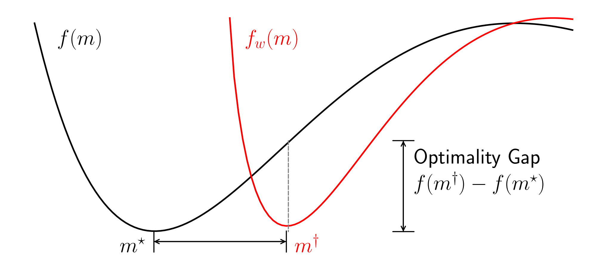
These bounds illustrate the need to control operator errors for surrogate derivatives as well as for their outputs.
Versions of this argument are made precise in the following results:
- Theorem 5 and Corollary 6 of our LazyDINO paper for inverse problems.
- Proposition 3.1 of our SISC paper for PDE-constrained optimization under uncertainty.
- Theorem 2.1, Proposition 2.2, and Theorems 3.1 and 3.2 of our shape DINO preprint for shape optimization.
- Propositions 2.1 and 2.2 of our DIFNO preprint for generic neural-operator-approximated deterministic optimization problems.
DINOs for Bayesian Inference
Results along these lines have been established for inverse problems, including our geometric MCMC paper and LazyDINO paper, led by my collaborator Lianghao Cao.
DINOS for PDE-constrained Optimization Under Uncertainty
Please see our SISC paper on efficient PDE-constrained optimization under uncertainty, led by my collaborator Dingcheng Luo, and our shape DINO preprint. We compare DINOs against conventional \(L^2_\mu\) neural operators (NO) and reference PDE solver based benchmark. Generally our results demonstrate that DINOs are \(10\times\) more accurate than NO and \(10 \times\) more sample efficient than reference PDE solver-based implementations when only amortized over one risk-averse optimization problem. When amortizing over many the benefits of DINO increase substantially.
DINOs are able to control viscous flow fields with expensive-to-estimate risk measures (CVaR) at \(\mathcal{O}(10^7)\) online speedup, with little loss of accuracy.
Uncontrolled flow field

Optimally controlled flow field

Application to 2011 Tōhoku earthquake
Through our NSF RISE grant, with collaborators Thorsten Becker, Simone Puel and Umberto Villa we are solving Bayesian inverse problems surrounding the 2011 M9 earthquake. Specifically we seek to infer the subsurface elastic properties as well as the fault slip, both under uncertainty.
